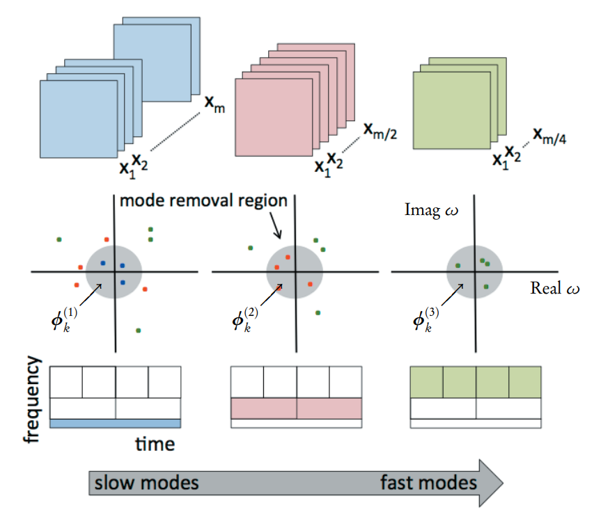
Plain DMD, as implemented in the previous page, is insensitive to translationally and rotationally invariant features, such as travelling waves. Multi-resolution DMD, or mrDMD, is one resolution, where the low-rank DMD modes are extracted successively using a recursive approach starting with m snapshots and decreasing by a factor of 2 at each resolution layer. An illustration of the method is shown in Figure 1.
A set of 100 continuous frames of disturbance waves past wall obstructions in a falling water film are used to apply DMD and mrDMD, and qualitatively compare their ability to detect these invariant features. The precise wave characteristics are unknown. A video of the images are shown below.
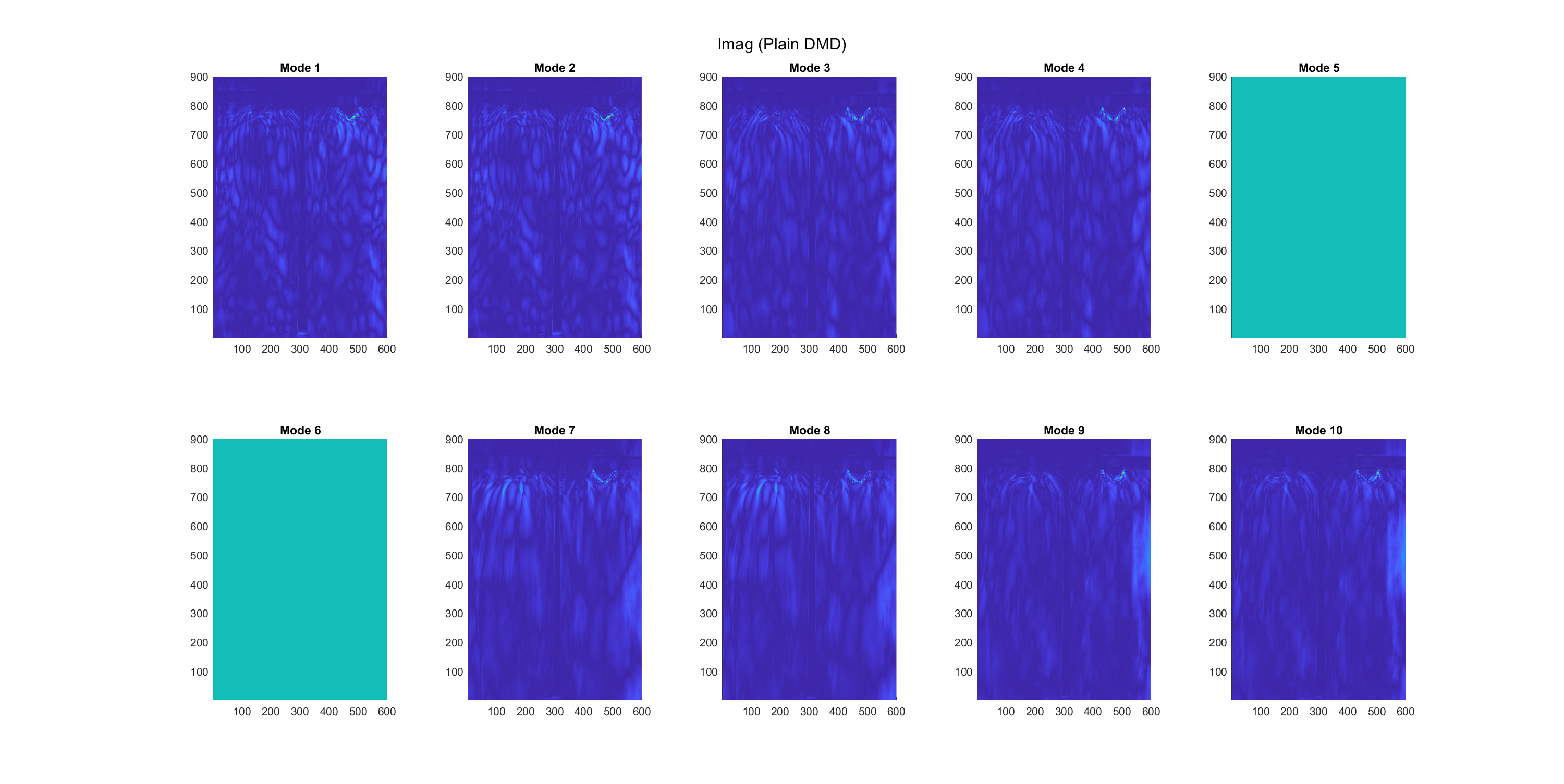
The real and imaginary parts of 10 modes, were extracted using the plain-DMD algorithm, as shown below in Figure 2 and 3, respectively. From the imaginary plots, which represent the phase shift of modes, modes 6 and 7 are static features, while all other modes are dynamic. This method does not show whether modes occur in any particular subset of the dataset, or throughout the dataset.
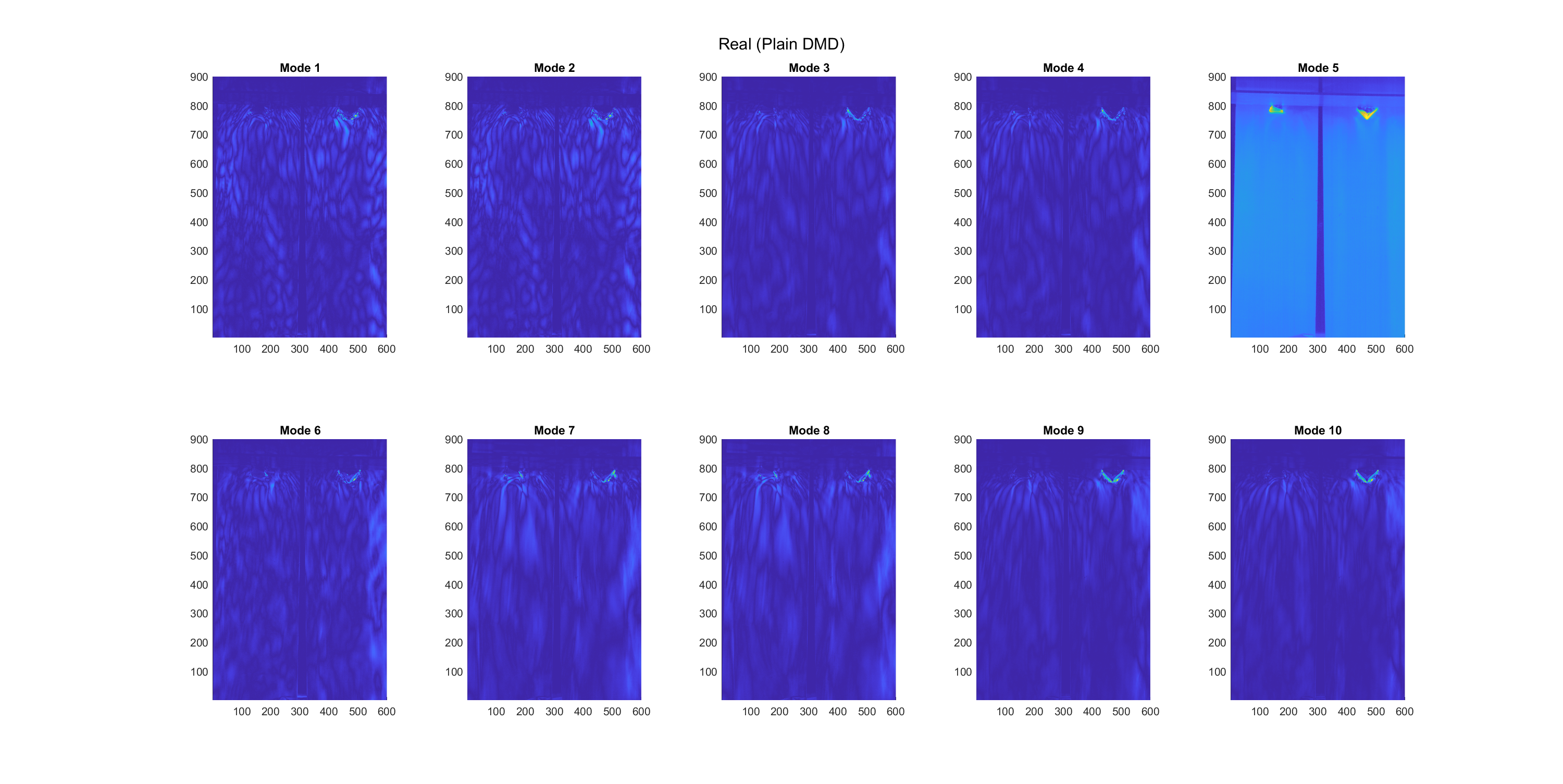
Figure 2. Real components of 10 plain-DMD modes in the falling film dataset.
The mrDMD algorithm is as follows:
%% mrDMD

function tree = mrDMD(Xraw, dt, r, max_cyc , L)

% Inputs:

% Xraw          n by m matrix of raw data,

%               n measurements, m snapshots

% dt            time step of sampling

% r             rank of truncation

% max_cyc       to determine rho , the freq cutoff , compute

%               oscillations of max_cyc in the time window

% L             number of levels remaining in the recursion
T = size(Xraw, 2) * dt;

rho = max_cyc/T; % high freq cutoff at this level

sub = ceil (1/rho/8/pi/dt); % 4x Nyquist for rho

%% DMD at this level

Xaug = Xraw (:, 1:sub:end); % subsample

Xaug = [Xaug(:, 1:end -1); Xaug(:, 2:end)];

X = Xaug(:, 1:end -1);

Xp = Xaug(:, 2:end);

[U, S, V] = svd(X, 'econ');

r = min(size (U,2), r);

U_r = U(:, 1:r); % rank truncation

S_r = S(1:r, 1:r);

V_r = V(:, 1:r);

Atilde = U_r' * Xp * V_r / S_r;

[W, D] = eig(Atilde);

lambda = diag(D);

Phi = Xp * V(:,1:r) / S(1:r,1:r) * W;
%% compute power of modes

Vand = zeros(r, size(X, 2)); % Vandermonde matrix

for k = 1:size(X, 2)

Vand(:, k) = lambda.^(k-1);

end
% the next 5 lines follow Jovanovic et al, 2014 code:

G = S_r * V_r';

P = (W'*W).*conj(Vand*Vand');

q = conj(diag(Vand *G'*W));

Pl = chol(P,'lower');

b = (Pl')\(Pl\q); % Optimal vector of amplitudes b
%% consolidate slow modes , where abs(omega) < rho

omega = log(lambda)/sub/dt/2/pi;

extractedModes = find(abs(omega) <= rho); thislevel.T = T; thislevel.rho = rho; thislevel.hit = numel(extractedModes) > 0;

thislevel.omega = omega(extractedModes);

thislevel.P = abs(b(extractedModes));

thislevel.Phi = Phi(:, extractedModes);
%% recurse on halves

if L > 1

sep = floor(size(Xraw ,2)/2);

nextlevel1 = mrDMD(Xraw(:, 1:sep),dt, r, max_cyc , L-1);

nextlevel2 = mrDMD(Xraw(:, sep+1:end),dt, r, max_cyc , L-1);

else

nextlevel1 = cell (0);

nextlevel2 = cell (0);

end
%% reconcile indexing on output

% (because MATLAB does not support recursive data structures)

tree = cell (L, 2^(L-1));

tree {1,1} = thislevel;

for l = 2:L

col = 1;

for j = 1:2^(l-2)

tree {l, col} = nextlevel1 {l-1, j};

col = col + 1;

end

for j = 1:2^(l-2)

tree {l, col} = nextlevel2 {l-1, j};

col = col + 1;

end

end
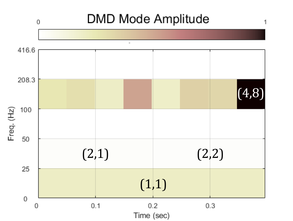
The real component of the mrDMD modes are shown in the gallery below, ordered by layer then by time. An schematic of the algorithm is shown in Figure 4. The amplitude of the 8th mode in the 4-th layer was the highest. All modes showed the time frame in which they occurred. This is a particularly different insight not provided by the plain DMD algorithm. By applying DMD to a successively smaller subset of the data, more sensitivity in the invariant features were observed while providing temporal specificity in the results.